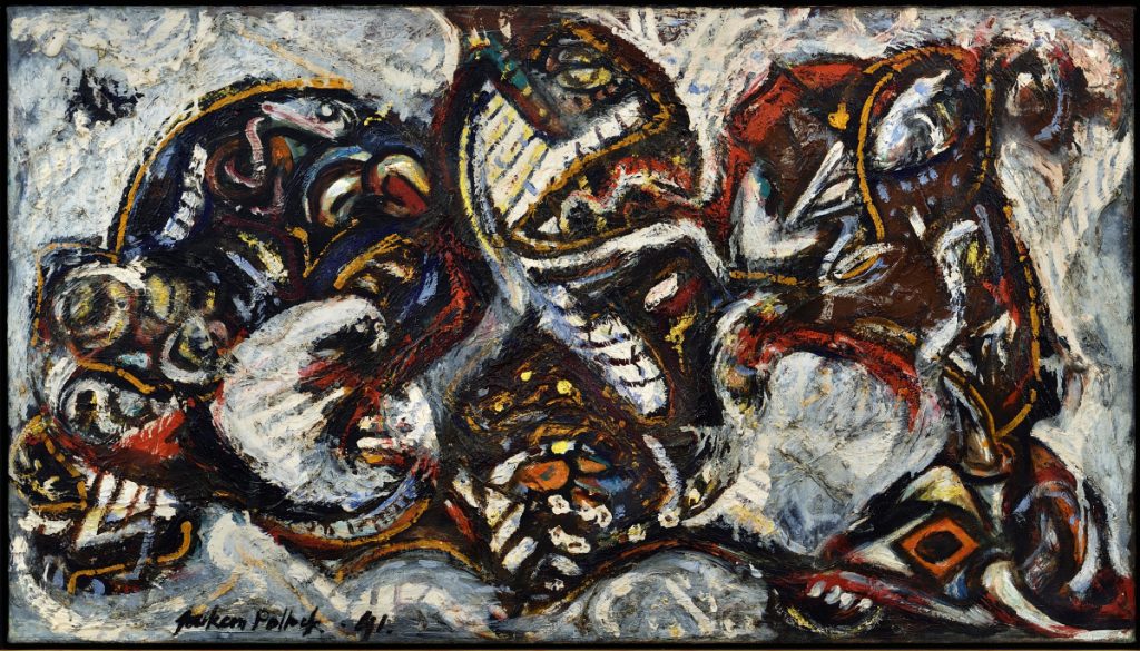
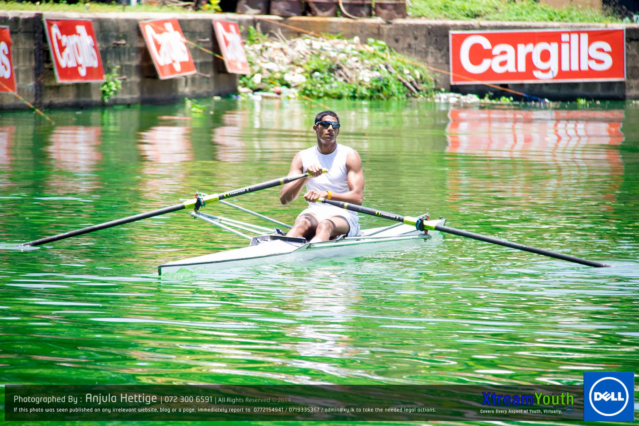
Performing Style Transfer Using a Convolutional Neural Network

In this documentation I will discuss the steps to take in implementing the style transfer algorithm. Style transfer allows you to apply the style of one image to another image of your choice. For example, here I have chosen a Salvador Dali painting for my style image, and I chose a rowing picture of myself for my Content image in order to produce this final style transfer image as shown below.

The key to this technique is using a trained CNN (Convolutional Neural Networks) to separate the content from the style of an image. If you can do this, then you can merge the content of one image, with the style of another and create something entirely different.

CNN’s process visual information in a feedforward manner; passing a input image through a collection of image filters, which extract certain features from the input image. It turns out that these feature level representations are not only useful for classification, but also for image construction like style transfer, which is based on CNN layer activations and extracted features.
Style transfer will look at two different images, we often call these the style image and the content image. Using a trained CNN, style transfer finds the style of one image and the content of the other. Finally, it tries to merge the two to create a new third image. In this newly created image, the objects and their arrangement are taken from the content image, and the colors and textures are taken from the style image.
For this style transfer process I used the features found in the 19 layer VGG Network (VGG 19). This network accepts a color image as input and passes it through a series of convolutional and pooling layers. Followed, finally by three fully connected layers that classify the passed-in image. In-between the five pooling layers, there are stacks of two or four convolutional layers. The depth of these layers is standard within each stack, but increases after each pooling layer.
In this process we’re not training the CNN at all. Rather our goal is to change only the target image, updating its appearance until it’s content representation matches that of our content image. So, we’re not using the VGG 19 network in a traditional sense, we’re not training it to produce a specific output. But we are using it as a feature extractor, and using back propagation to minimize a defined loss function between our target and content images. In fact, we’ll have to define a loss function between our target and style images, in order to produce an image with our desired style.
We look at how similar the features in a single layer are. Similarities will include the general colors and textures found in that layer. We typically find the similarities between features in multiple layers in the network. By including the correlations between multiple layers of different sizes, we can obtain a multi-scale style representation of the input image; one that captures large and small style features. Here, the correlations at each layer are given by a Gram Matrix, where the matrix is a result of a couple of operations. (Note - Gram Matrix is just one mathematical way of representing the idea of shared in prominent styles. Style itself is an abstract idea, but the Gram Matrix is the most widely used in practice.)
We change the Target image’s style representations as we minimize this loss over some number of iterations. By calculating the content loss, which tells us how close the content of our target image is to that of our content image and the style loss, which tells us how close our target is in style to our style image; we add these losses together to get the total loss, and then use typical back propagation and optimization to reduce this loss by iteratively changing the target image to match our desired content and style.
We have values for the content and style loss, but since they are calculated differently, these values will be pretty different, and we want our target image to take both into account fairly equally. It’s necessary to apply constant weights, alpha and beta, to content and style losses respectively. Such that the total loss reflects in equal balance. In practice, this means multiplying the style loss by a much larger weight value than the content loss. You’ll often see this expressed as a ratio of the content and style weights, alpha over beta. It is recommended that the smaller the alpha-beta ratio, the more stylistic effect you will see.

Implementing Style Transfer with Deep Neural Networks Using PyTorch

Here, I have used a pre-trained VGG 19 net as a feature extractor. We can put individual images through this network, then at specific layers get the output, and calculate the content and style representations for an image. With the code shown below, you’ll be able to upload images of your own and really customize your own target style image.

First, we will go ahead and load in our libraries.

 # import libraries
 from PIL import Image
 import matplotlib.pyplot as plt
 import numpy as np

 import torch
 import torch.optim as optim
 from torchvision import transforms, models

Next, we will load in the pre-trained VGG 19 network that this implementation relies on. Using PyTorch’s models we can load this network in by name and ask for it to be pre-trained. We actually just want to load in all the convolutional and pooling layers, which in this case are named as features, and this is unique to the VGG network. Here, we will load in a model and we will freeze any weights or parameters that we don’t want to change. So, we are saving this pre-trained model using the VGG variable, then for every weight in this network we are setting requires_grad to False. This means that none of these weights will change. Hence, VGG becomes a kind of fixed feature extractor, which is just what we want for getting content and style features later.

 # getting features of VGG 19
 vgg = models.vgg19(pretrained=True).features

 # freezing all VGG weights and parameters to optimize for target image only
 for param in vgg.parameters():
     param.requires_grad_(False)

Next, we will check if a GPU device is available, and if it is, we will move our model to it in order to speed up the target image creation process. Here, vgg.to(device) will print out the VGG model and all it’s layers. (Once printed out on console, you will notice that the sequence of all layers is numbered)

 # move to GPU... if available, if not use CPU for slower process lol
 device = torch.device("cuda" if torch.cuda.is_available() else "cpu")

 vgg.to(device)

Here, we have our trained VGG model and now we need to load in our content and style images. Below we have a function which will transform any image into a normalized tensor. This will deal with jpg, png or some image format, and it will make sure that the size is reasonable for our purpose.

 def load_image(img_path, max_size=400, shape=None):
     ''' Load in and transform an image, making sure the image
        is <= 400 pixels in the x-y dims.'''

     image = Image.open(img_path).convert('RGB')

     # process will slow down if image is large
     if max(image.size) > max_size:
         size = max_size
     else:
         size = max(image.size)

     if shape is not None:
         size = shape

     in_transform = transforms.Compose([
                         transforms.Resize(size),
                         transforms.ToTensor(),
                         transforms.Normalize((0.485, 0.456, 0.406),
                                              (0.229, 0.224, 0.225))])

     image = in_transform(image)[:3,:,:].unsqueeze(0)

     return image

Here, we will load in style and content images from our images directory. Here, we will reshape out style image into the same shape as the content image. This reshaping step is just going to make the math nicely lined up later on.

 # load in content image and style image
 content = load_image('images/rowing.jpg').to(device)
 style = load_image('images/memory.jpg', shape=content.shape[-2:]).to(device)

Next, we will also have a function to help us convert a normalized tensor image back into a numpy image for display. Here, I can show you the images that I choose. I chose a rowing picture of myself for my Content image and a Salvador Dali painting for my style image.

 # convert Tensor image to NumPy image -- to display
 def im_convert(tensor):
     """ Display a tensor as an image. """

     image = tensor.to("cpu").clone().detach()
     image = image.numpy().squeeze()
     image = image.transpose(1,2,0)
     image = image * np.array((0.229, 0.224, 0.225)) + np.array((0.485, 0.456, 0.406))
     image = image.clip(0, 1)

     return image

Next, we know we eventually have to pass our content and style images through our VGG network, and extract content and style features from particular layers. Below, the get_features function takes in an image and returns the outputs from layers that correspond to our content and style representations. This is going to be a list of features that are taken at particular layers in our VGG 19 model.

 def get_features(image, model, layers=None):
     #Runs an image in a feedforward through a model and get the features for each layer
     if layers is None:
         layers = {'0': 'conv1_1',
                   '5': 'conv2_1',
                   '10': 'conv3_1',
                   '19': 'conv4_1',
                   '21': 'conv4_2',  
                   '28': 'conv5_1'}

     features = {}
     x = image

     for name, layer in model._modules.items():
         x = layer(x)
         if name in layers:
             features[layers[name]] = x

     return features

(Note - The descriptive dictionary maps our VGG 19 layers, that are currently numbered from 0 through 36, into names like conv1_1, conv2_1 and so on.)

Next, we need to pass a style image through the VGG model and extract the style features at the right layers which we’ve just specified. Then, once we get these style features at a specific layer, we’ll have to compute the Gram Matrix. This function takes in a tensor, which will be the output of some convolutional layer, and returns the Gram Matrix, the correlations of all the features in that layer. Here, we are ignoring the batch size, since we are only interested in the depth (number of feature maps), height and width. Next, we reshape the tensor to a 2D shape and then we calculate the Gram Matrix by multiplying this Tensor times it’s transpose and we return the calculated Matrix.

 def gram_matrix(tensor):
     # Get depth, height, and width of Tensor
     _, d, h, w = tensor.size()
     # Reshaping tensor
     tensor = tensor.view(d, h * w)
     # Calculate Gram Matrix
     gram = torch.mm(tensor, tensor.t())
     return gram

Next, we will put all the functions together. In the below code, we call get_features on our content image, passing in our content image and the VGG model; we do the same thing for our style features as well, passing in our style image and the VGG model. The style_grams variable will look at all of the layers in our style features and will compute the Gram Matrix. We will start our target image as a clone of our content image, and then iteratively change the target image.

 # Get content and style features only once since we want these to remain the same throughout this process
 content_features = get_features(content, vgg)
 style_features = get_features(style, vgg)
 # Calculating Gram Matrix for each layer
 style_grams = {layer: gram_matrix(style_features[layer]) for layer in style_features}
 # Here, create a Target image, starting our target image as a clone of our content image, later iteratively changing by style
 target = content.clone().requires_grad_(True).to(device)

Here, we will calculate our style and content losses for creating interesting target images. We can play around with the values for the style_weights giving more weight to earlier layers (It is preference to weigh earlier layers higher and it is recommended to keep values within the zero to one range). Next, we will give our content (alpha) and style (beta) weight. Because of how style loss is calculated, we basically want to give our style loss a much larger weight than the content loss (if beta is too large, you may see too much of a stylized effect).

style_weights = {'conv1_1': 1.,
                 'conv2_1': 0.75,
                 'conv3_1': 0.2,
                 'conv4_1': 0.2,
                 'conv5_1': 0.2}

content_weight = 1  # Alpha
style_weight = 1e6  # Beta

Next, we enter the iteration loop. Here is where we will actually change our target image. Now, keep in mind this is not a training process, hence, it’s arbitrary where we stop updating the target image. It is recommended to have at least 2000 iterations. But you may want to do more or less depending on your computing resources and desired effect. Here, I ran this loop for 2000 iterations, but I showed intermittently images every 400. The loss was also printed out with the image which seemed to be quite large and a difference could be seen in my rowing image right away. (Note - In the iteration loop, when calculating the content loss, we will mean square the difference between the target and content representations. We can get those representations by getting the features from our target image, and then comparing those features at a particular layer, in this case conv4_2, to the features at that layer for our content image. We’re going to subtract these two representations and square that difference and calculate the mean. This will give us our content loss. Next, in this loop we do something similar for the style loss. Only this time we have to go through multiple layers for our multiple representations for style. Recall that each of our relevant layers was listed in our style_weights dictionary above.)

# Display target image every 400 iterations
show_every = 400

# iteration hyper-parameters
optimizer = optim.Adam([target], lr=0.003)
steps = 2000  # define Iterations needed to update target image

for ii in range(1, steps+1):

    # Getting features from target image
    target_features = get_features(target, vgg)

    # Calculating Content Loss
    content_loss = torch.mean((target_features['conv4_2'] - content_features['conv4_2'])**2)

    # Calculating style loss and initializing it to zero and later adding it to each layer's gram matrix loss
    style_loss = 0

    for layer in style_weights:
        # Getting target style representation
        target_feature = target_features[layer]
        target_gram = gram_matrix(target_feature)
        _, d, h, w = target_feature.shape
        # Getting the style of the style image representation
        style_gram = style_grams[layer]
        # Calculating style loss of one layer
        layer_style_loss = style_weights[layer] * torch.mean((target_gram - style_gram)**2)
        # adding the style loss of previous step to total style loss
        style_loss += layer_style_loss / (d * h * w)

    # calculating the total loss
    total_loss = content_weight * content_loss + style_weight * style_loss

    # Updating target image
    optimizer.zero_grad()
    total_loss.backward()
    optimizer.step()

    # Displaying the target image every 400 iterations and printing total loss
    if  ii % show_every == 0:
        print('Total loss: ', total_loss.item())
        plt.imshow(im_convert(target))
        plt.show()

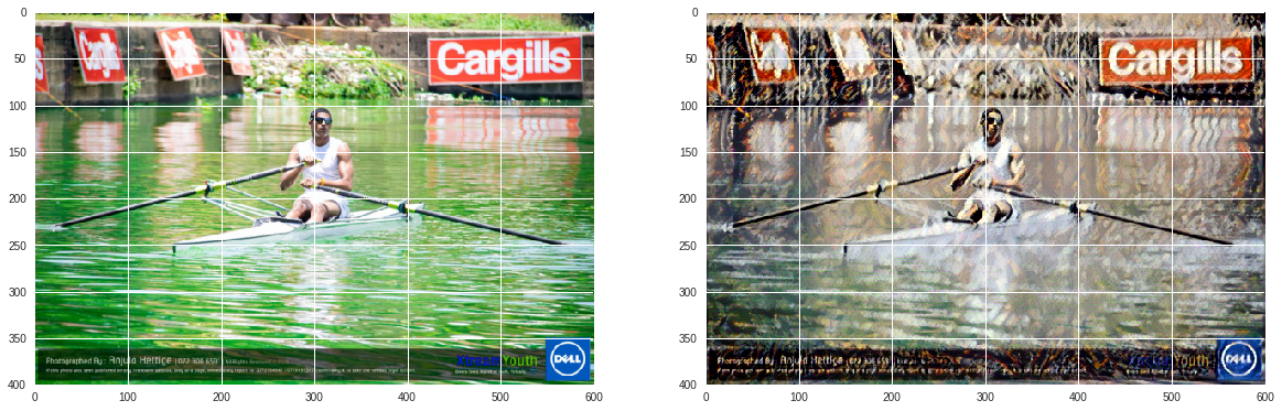
Then at the end of my 2000 iterations, I displayed my content, and my target image side-by-side. You can see that the target image still looks a lot like the content image. However, I think I could have stylized this even more. If you look closely you will notice that the target image has some of the brushstroke texture from the Salvador Dali painting which was used as my style image.

# Display both content and final image side by side
fig, (ax1, ax2) = plt.subplots(1, 2, figsize=(20, 10))
ax1.imshow(im_convert(content))
ax2.imshow(im_convert(target))

Performing Style Transfer Using a Convolutional Neural Network

CATALOG

FEATURED TAGS